Monte Carlo Radiation Transport
Radiation moving through matter is described by, among others, the linear Boltzmann transport equation: streaming, scattering, absorption, and production of secondary particles. For any geometry you actually care about (a shield with penetrations and welds, a detector with crystals, reflectors, and dead layers) it has no closed-form solution. So you sample it instead, with Monte Carlo.
I took the intro to MCNP class at Los Alamos in 2010 and used MCNP (Monte Carlo N-Particle) for a good chunk of my thesis and my work at LLNL, producing several papers with it (Google Scholar).
Where the method came from
The method is almost exactly as old as electronic computing, and the two grew up together for the same job: simulating neutrons for the bomb. While recovering from an illness at Los Alamos in 1946, Stanislaw Ulam was playing solitaire and wondered what the odds of winning a hand actually were. The combinatorics were hopeless by hand, but you could just deal a lot of hands and count. The same trick worked for neutrons diffusing through fissile material: too tangled to solve analytically, easy to sample. John von Neumann wrote it up as a computation for ENIAC, one of the first electronic computers, and by 1948 it was running neutron transport for the weapons program. Nicholas Metropolis named it Monte Carlo, after the casino where Ulam's uncle gambled.
That lineage never stopped. MCNP descends directly from those first Los Alamos neutron codes, which makes it one of the oldest continuously developed pieces of software anywhere, with predecessors going back to the late 1940s.
The idea
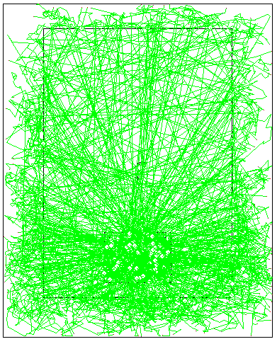
Instead of solving the equation, you simulate one particle's life as a sequence of random choices, then repeat it a few million times and average. You are not coarse-meshing the equation and hoping; you are sampling the same distributions the equation is built from: distance to the next interaction (from the mean free path), scatter versus absorption, and the new direction and energy after a scatter. Each is a known distribution from the nuclear data. Follow enough histories and the law of large numbers converges on the answer, with a quantified error.
 hover / hold for original
How MCNP works
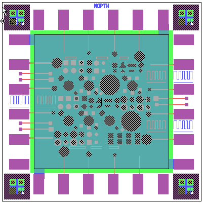
You write a deck, a plain-text input with a few jobs. That vocabulary is itself a relic: the input is a "deck" and each line in it is a "card," left over from when a program was a literal stack of punched cards you carried to the machine. The deck still has a few kinds of card:
- Geometry. Define surfaces (planes, spheres, cylinders) and combine them with Boolean logic into cells. Combinatorial geometry is powerful and the most common source of error: leave a gap or overlap two cells and particles are lost to the void.
- Materials. Each cell gets isotopes, densities, and cross-section libraries. The result is only as good as the nuclear data.
- Source. Particle type, energy, position, and direction: a Cf-252 point source, a beam, a distributed volume source.
- Tallies. What you want to score: surface flux, energy deposition, current, dose. The tally is the question.
Particles random-walk through the geometry and the tallies accumulate. Every result comes with a relative error, because it is a statistical estimate.
 hover / hold for original
Variance reduction
Statistical error falls as one over the square root of the history count: a 10x improvement costs 100x the particles. That is brutal for deep-penetration problems, where most source particles die long before reaching the tally. Variance reduction biases the simulation toward the histories that contribute and corrects with statistical weights to keep the estimate unbiased. The standard tools are importance with particle splitting and Russian roulette, and weight windows (a spatially varying, automated version). Done well, a week-long run finishes overnight; done badly, you bias the answer or wreck the statistics. This is most of the actual skill.
The error bars are the result
A Monte Carlo mean without a converged error estimate is not a result. MCNP runs ten statistical checks per tally: relative error magnitude, 1/sqrt(N) behavior, a stable figure of merit, and the variance of the variance. The dangerous failure is a clean-looking mean sitting on unconverged statistics, usually one rare high-weight history dominating the tally. Check the diagnostics, not just the number.
 hover / hold for original
What it is for
Shielding design, occupational and public dose, predicting detector response, and criticality safety. When you cannot build it and measure, you simulate.
MCNP is export-controlled and distributed through RSICC, which makes it a poor teaching tool. When I needed something students could install and run themselves I used the open-source alternative, which I wrote about in teaching with GEANT4. For transport work that needs an experienced hand, that is one of the things I take on at Such Software.